Cost Minimization Curves
Output Expansion Path
- The output expansion path is the curve containing the cost-minizing input bundles at differing levels of output
- Analagous to the price offer curve on the demand side
- Can only exist in the long-run where all costs are variable

- The conditional input demand curve plots the conditional input demand against output
- Analagous to the Engel curve on the demand side
- y-axis would have output y, x-axis would have input xi
Fixed-Proportions Technology Curves
y=min{4x1,x2}4x1∗=x2∗=yx1∗(w1,w2,y)=y/4x2∗(w1,w2,y)=y
In this situation, you would choose bundles at the vertices of the L-shaped isoquants.
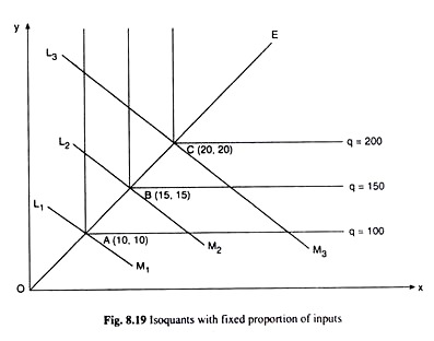
The firm’s total cost function is therefore: c(w1,w2,y)=w1x1∗(w1,w2,y)+w2x2∗(w1,w2,y)=w14y+w2y=(4w1+w2)y
Perfect Substitutes Technology Curves
Depending on whether or not the slopes of the isocost and isoquant are the same, there could be infinitely many solutions (slopes equal) or one corner solution (slopes unequal).
y=x1+2x2,MP2MP1=1/2Three cases:If w1/w2>1/2, then x1∗=0,x2∗=y/2,c(w1,w2,y)=2yw2If w1/w2<1/2, then x1∗=y,x2∗=0,c(w1,w2,y)=yw1If w1/w2=1/2, then any bundle on the isoquant can be chosen.Thus, c(w1,w2,y)=min{yw1,2yw2}=y⋅min{w1,2w2}
Cost Curves
Average Cost
- For a positive y, a firm’s average cost of producing y output units is AC(w1, w2, y) = c(w1, w2, y) / y
- This is also known as cost per unit of output
- Given constant RTS, doubling the output level from y’ to 2y’ requires doubling all input levels. Thus, the AC does not change, as both c and y are multiplied by 2
- Given decreasing RTS, doubling the output level from y’ to 2y’ requires more than doubling all input levels. Thus, the AC increases, as c increases at a higher rate than y
- Given increasing RTS, doubling the output level from y’ to 2y’ requires less than doubling all input levels. Thus, the AC decreases, as y increases at a higher rate than c
Short Run and Long Run Total Costs
The LR cost minization problem minimizes w1x1+w2x2, x1,x2≥0 such that f(x1,x2)=yThe SR cost minization problem minimizes w1x1+w2x2′, x1≥0 such that f(x1,x2′)=yThe SR problem can be rewritten as w1x1+w2x2, x1,x2≥0 such that f(x1,x2)=y,x2=x2′
- Note that this means that SR total cost will exceed LR total cost except for the output level where the SR input level restriction is the same as the LR input level choice