Cost Minimization
- A firm is a cost minimizer if it produces any given output level (y > 0) with the smallest possible total cost
- Note that factor and input are synonyms in this chapter; they are interchangable
When the firm faces given input prices w=(w1,w2,...,wn)the total cost function will be written as c(w1,...,wn,y)
- Note that the total cost function does not include the amounts of inputs; this is because the total cost function is implied to use the optimal amount of inputs to minimize costs
- In other words, the total cost function gives the firm’s smallest possible total cost for producing y units of output given input prices w = (w1, …, wn)
Cost Minimization Problem
- Given two inputs and one output, we get the production function y = f(x1, x2)
- Given the input prices w1, w2, the cost of an input bundle (x1, x2) is w1x1 + w2x2
Given w1,w2,y, the firm’s cost minimization problem is min{w1x1+w2x2} such that f(x1,x2)=y
The levels x1*(w1, w2, y) and x2*(w1, w2, y) in the least costly input bundle are the firm’s conditional demands for inputs 1 and 2.
The smallest possible total cost for producing y output units is therefore c(w1, w2, y) = w1x1*(w1, w2, y) + w2x2*(w1, w2, y)
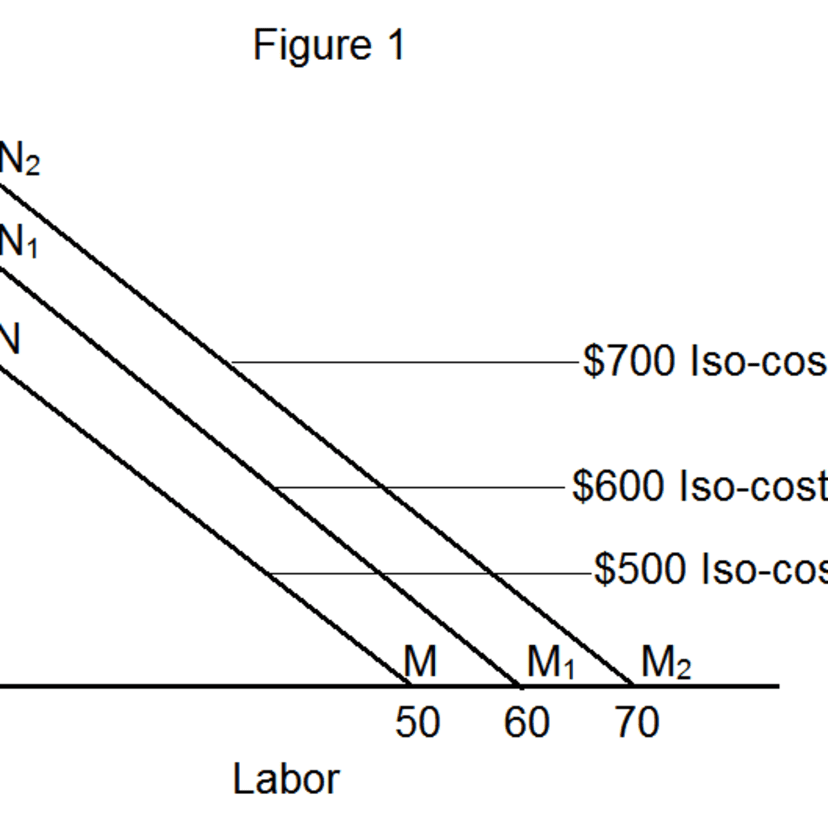
Isocost Lines
- An isocost curve contains all the input bundles that cost the same amount
- The isocost curve is extremely similar to the budget constraint, even sharing similar equations
Given w1 and w2, the equation of an isocost line with a cost of c is w1x1+w2x2=cThis can also be written as x2=−w2w1x1+w2c
- The graph of isocost lines is therefore a series of parallel lines, with lower costs being closer to the origin
- To minimize costs, we must find the lowest possible isocost line that is tangent with the isoquant curve corresponding to a given output level

- To find the cost minizing bundle, set the slope (TRS) of the isoquant curve equal to the slope of the isocost curve
At an interior cost-minimizing input bundle:f(x1∗,x2∗)=y′Slope of isocost = slope of isoquant, or −w2w1=TRS=−MP2MP1 at (x1∗,x2∗)
Cobb-Douglas Example
y=f(x1,x2)=x11/3x22/3 with input prices w1,w2Must satisfy two conditions: y=x11/3x22/3−w2w1=−MP2MP1=2x1∗x2∗From the second condition: x2∗=w22w1x1∗y=(x1∗)1/3(w22w1x1∗)2/3=x1∗(w22w1)2/3x1∗=y(2w1w2)2/3x2∗=w22w1y(2w1w2)2/3=(w22w1)1/3y