Isoquant Curves and Choosing Bundles

Isoquant Curves

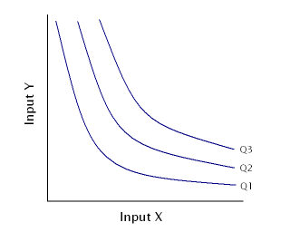
• An isoquant is defined as the set of all input bundles (x₁, x₂) that are just sufficient to produce a given amount of output y

• The complete collection of isoquants is the isoquant map

  • Note that production levels are different than utility levels; while utility levels are only ordinal (i.e. you only care about perserving the order of preference relations), the actual numbers of the production levels matter because they map to the amount a supplier is able to produce

$$\text{Cobb-Douglas Technologies take on the following form:}\\ y = Ax_1 ^{a_1} \cdot ... \cdot x_n ^{a_n} \\ \text{Ex: } y = x_1^{1/3}x_2^{1/3} \\ \text{Fixed-Proportions Technologies (analagous to perfect complements) take on the following form:}\\ y = min\{a_1 x_1, ..., a_n x_n\} \\ \text{Ex: } y = min\{x_1, 2x_2\} \\ \text{Perfect-Substitutes Technologies take on the following form:}\\ y = a_1 x_1 + ... + a_n x_n \\ \text{Ex: } y = x_1 + 3x_2$$

• The graphs for all of these isoquants are the same as their indifference curve counterparts; Cobb-Douglas are curved, Fixed-Proportions are L-shaped, Perfect-Substitutes are parallel + linear

Marginal Products

• The marginal (physical) product of input i is the rate-of-change of the output level as the level of input i changes, holding all other input levels fixed
• The marginal revenue product is equal to the marginal product times the price of the output

$$MP_i = \frac{\partial y}{\partial x_i} \\ \text{Cobb-Douglas Example: } y = x_1^{1/3}x_2^{2/3} \\ MP_1 = \frac{\partial y}{\partial x_1} = \frac{1}{3} x_1^{-2/3}x_2^{2/3} \\ MP_1 = \frac{\partial y}{\partial x_2} = \frac{2}{3} x_1^{1/3}x_2^{-1/3}$$ $$MP_i \text{ is diminishing if it becomes smaller as } x_i \text{ increases.} \\ \text{That is, if } \frac{\partial MP_i}{\partial x_1} = \frac{\partial}{\partial x_i} \frac{\partial y}{\partial x_i} = \frac{\partial^2 y}{\partial x_i^2} < 0 \\ \text{Note that the coefficient of the second derivative determines whether or not the MP is diminishing,} \\ \text{as the inputs } x_i \text{ are non-negative.}$$

Returns-to-Scale

• The MP describes the rate-of-change in output level as a single input level changes; however, returns-to-scale describes the rate-of-change in output level as all input levels change in direct proportion, such as when all input levels double or half

$$\text{If, for any input bundle, } f(kx_1, ..., kx_n) = kf(x_1, ..., x_n) \text{ for all k > 1,} \\ \text{then the technology exhibits constant RTS.} \\ \text{If } f(kx_1, ..., kx_n) < kf(x_1, ..., x_n) \text{, then the technology exhibits decreasing RTS.} \\ \text{If } f(kx_1, ..., kx_n) > kf(x_1, ..., x_n) \text{, then the technology exhibits increasing RTS.} \\$$

• A production function with one input and one output will be linear if constant RTS, increasing at decreasing rate if decreasing RTS, and increasing at increasing rate if increasing RTS
  • Note that RTS is dependent on the second derivative, so one technology can have different RTS depending on its second derivative
  • A technology can not have permenant increasing RTS
• Perfect-Substitutes have a constant RTS, Fixed-Proportions have a constant RTS, Cobb-Douglas depends on the exponents
  • For Cobb-Douglas, if the sum of the exponents equals one, then the production has constant RTS. Less than 1 means decreasing and greater than 1 means increasing

$$\text{Showing how Cobb-Douglas exponents determine the RTS:}\\ y = x_1^{a_1} \cdot ... \cdot x_n^{a_n} \\ ky = (kx_1)^{a_1} \cdot ... \cdot (kx_n)^{a_n} \\ ky = k^{a_1 + ... + a_n}x_1^{a_1} \cdot ... \cdot x_n^{a_n}$$